
When you work with a lot of data in Google Sheets, it is very common to accidentally get duplicate entries. Duplicate entries are rows or cells that contain the exact same information more than once. Having duplicates can make your totals wrong and your spreadsheets look messy.
Thankfully, cleaning up your data is very easy. Google Sheets gives you two excellent ways to handle this problem. The first way deletes the duplicates permanently, and the second way creates a clean list in a new spot without changing your original data.
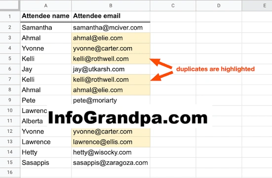
Here is a simple, step-by-step guide to both methods.
Method 1: The “How to Remove Duplicate Google Sheets ” Tool (Permanent Cleanup)
Use this method if you want to completely get rid of the duplicate rows and you do not need to keep them anymore.
Stp 1: Select your data
Click and hold your mouse, then drag it over all the cells you want to check. If you want to select your entire spreadsheet quickly, press Ctrl + A on a Windows computer or Cmd + A on a Mac.
Step 2: Open the Cleanup Tool
Look at the top menu bar of your Google Sheet. Click on the word Data. A dropdown menu will appear. Move your mouse down to Data cleanup, and then click on Remove duplicates.
Step 3: Choose your settings
A small settings box will pop up on your screen. It will ask you a couple of questions:
- Data has header row: Check this box if the very first row of your sheet has titles (like “Name”, “Date”, or “Email”). Checking this protects your titles so Google Sheets does not accidentally delete them.
- Columns to analyze: Decide if you want to look at the whole sheet or just one column. If you leave “Select all” checked, Google Sheets will only delete a row if the entire row matches another one exactly. If you uncheck it and pick just one column (like “Email”), it will delete any row that has a repeated email address.
Step 4: Delete the duplicates
Click the blue button that says Remove duplicates. A small message will pop up telling you exactly how many duplicate rows were found and removed. Click OK to finish.
Method 2: The UNIQUE Formula (Safe and Dynamic)
Use this method if you are worried about deleting your original data and want to keep it exactly as it is. This formula looks at your messy data and copies only the unique items to a brand-new section of your sheet.
Step 1: Find an empty space
Look for an empty column or a completely blank area on your spreadsheet where you have plenty of room. Click into the top cell of that empty area.
Step 2: Type the formula
Type =UNIQUE( into the cell.
Step 3: Select your messy data range
Type or select the range of cells you want to clean up. For example, if your data starts at cell A1 and goes down to cell C100, your formula should look like this: =UNIQUE(A1:C100)
Step 4: Press Enter
Press the Enter key on your keyboard. Google Sheets will instantly generate a clean list of data without any duplicates.
The best part about this method is that it is “live.” If you add more data to your original list later, the UNIQUE formula will automatically update your clean list!
Which Method Should You Use?
- Choose Method 1 (The Tool) if you are completely finished with your data and want a permanent, quick cleanup.
- Choose Method 2 (The Formula) if you want to keep your original list safe, or if you plan on adding more information to your spreadsheet later.
With these two simple tools, you can keep your spreadsheets accurate, clean, and organized!
More on InfoGrandpa.com:
A Guide to Setting Up an Effective Classroom Center